Category Theory
Table of Contents
- 1. Category
- 2. Morphism
- 3. Functor
- 4. Commutative Diagram
- 5. Natural Transformation
- 6. Product
- 7. Equaliser
- 8. Diagram
- 9. Limit
- 10. Universal Property
- 11. Yoneda Lemma
- 12. Sheaf
- 13. Monad
- 14. Monoidal Category
- 15. See Also
- 16. References
- Category theory is an abstraction of structure.
- Abstract algebra with structures between abstract objects. The abstract objects and morphisms form a category.
1. Category
1.1. Definition
A category \(\mathcal C\) consists of
- a set of objects \(\mathrm{ob}(\mathcal C)\)
- sets of morphisms \(\mathrm{Hom}_{\mathcal{C}}(A,B)\) called homsets between each pair of objects \(A,B\) in \(\mathcal{C}\)
- binary operation \(\circ\colon \mathrm{Hom}_{\mathcal{C}}(B, C)\times\mathrm{Hom}_{\mathcal{C}}(A, B)\to \mathrm{Hom}_{\mathcal{C}}(A, C)\) called composition of morphisms
satifying the following properties:
- Identity: \(\forall\,X \in \mathcal{C},\exists\, \mathrm{id}_{X}:X\to X\), such that for \(f\in \mathrm{Hom}_{\mathcal{C}}(A,X)\) and \(g\in \mathrm{Hom}_{\mathcal{C}}(X,A)\), \(f\circ \mathrm{id}_{X}=f\) and \(\mathrm{id}_{X}\circ g= g\) holds.
- Associativity: If \(f\in \mathrm{Hom}(A, B), g\in\mathrm{Hom}(B, C), h\in\mathrm{Hom}(C, D)\), then \(h\circ(g\circ f) = (h\circ g)\circ f.\)
1.2. Classification
1.2.1. Small Category
If the set of objects \( \mathrm{ob}(\mathcal{C}) \) is not a proper class.
1.2.2. Locally Small Category
If the homsets \( \mathrm{Hom}_{\mathcal{C}}(A, B) \) are not a proper class.
1.3. Discrete Category
A category whose only morphisms are the identity morphisms: \[ \mathrm{Hom}_{\mathcal{C}}(X, Y) = \begin{cases} \{\mathrm{id}_X\} & \text{if $X=Y$,}\\ \varnothing & \text{if $X\neq Y$.} \end{cases} \]
1.4. Functor Category
The class of functors from \(\mathcal{C}\) to \(\mathcal{D}\) with morphisms being the natural transformations. It is commonly written as \( \mathcal{D}^\mathcal{C} \).
1.5. Opposite Category
- Dual Category
An opposite category \( \mathcal{C}^{\mathrm{op}} \) is a category where all the arrows are reversed from a given category \( \mathcal{C} \).
1.6. Thin Category
- Posetal Category, (0,1)-Category
A category is called thin, if there are at most one morphism in each homset.
This can effectively represent the sturcture of a poset (partially ordered set). One example of this is the category of open sets \( \mathrm{Op}(X) \) of a topological space \( X \), in which the inclusions \( \iota\colon V \hookrightarrow U \) are the morphisms.
2. Morphism
2.1. Classification
2.1.1. Monomorphism
- \(\hookrightarrow\) (Inclusion), \(\rightarrowtail\) (Injection)
Monic Morphism, Mono
A left-cancellative morphism such that: \[ f\circ g_1 = f\circ g_2 \implies g_1 = g_2 \]
2.1.1.1. Regular Monomorphism
Monomorphism that are also an equaliser.
2.1.1.2. Extremal Monomorphism
A monomorphism \( \mu \) that \(\mu = \varphi \circ \varepsilon\land \varepsilon\text{ epimorphism} \implies \varepsilon\text{ isomorphism}\)
2.1.1.3. Immediate Monomorphism
- \(\mu = \mu' \circ \varepsilon\land \mu'\text{ monomorphism} \land \varepsilon\text{ epimorphism} \implies \varepsilon\text{ isomorphism}\)
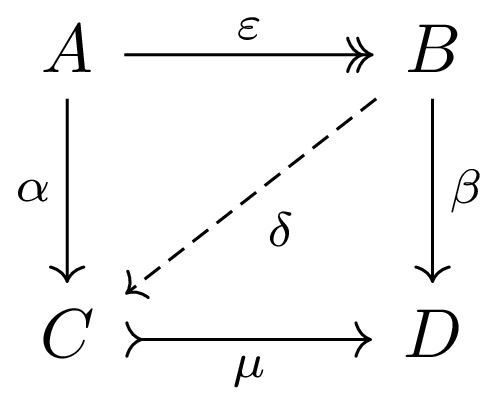
2.1.1.4. Strong Monomorphism
A monomorphism \(\mu\) is called strong if for any epimorphism \( \varepsilon \) and any morphisms \( \alpha, \beta \), there exists a morphism \( \delta \) that makes the following diagram commute:
2.1.1.5. Split Momomorphism
- \(\exists \varepsilon : \varepsilon \circ \mu = 1\)
2.1.2. Epimorphism
- \(\twoheadrightarrow\) (Surjection, Projection)
- Epic Morphism
A right-cancellative morphism \( f \) such that: \[ g_1\circ f = g_2\circ f \implies g_1 = g_2. \]
2.1.2.1. Regular Epimorphism
An epimorphism that is also a coequaliser.
2.1.2.2. Extremal Epimorphism
- \(\varepsilon = \mu \circ \varphi \land \mu\text{ monomorphism} \implies \mu\text{ isomorphism}\)
2.1.2.3. Immediate Epimorphism
- \(\varepsilon = \mu \circ \varepsilon'\land \mu\text{ monomorphism}\land \varepsilon'\text{ epimorphism} \implies \varepsilon\text{ isomorphism}\)
2.1.2.4. Strong Epimorphism
An epimorphism \(\varepsilon\) is called strong if for any monomorphism \( \mu \) and any morphisms \( \alpha, \beta \), there exists a morphism \( \delta \) that makes the following diagram commute:
2.1.2.5. Split Epimorphism
- \(\exists \mu : \varepsilon \circ \mu = 1\)
2.1.3. Bimorphism
- \(\mathrel{\rightarrowtail\kern-10pt\twoheadrightarrow}\)
- Both monomorphism and epimorphism
2.1.4. Isomorphism
- \(\xrightarrow{\mathpunct{\sim}}\)
- \(\exists g : g\circ f = 1_X \land f\circ g = 1_Y\)
- See isomorphism.
2.1.5. Endomorphism
- \(\mathrm{End}(X)\)
- \(f\colon X\to X\)
2.1.6. Automorphism
- Both endomorphism and isomorphism
2.1.7. Retraction
- Right inverse exists
- \(\exists g : f\circ g = 1_Y\)
2.1.8. Section
- Left inverse exists
- \(\exists g : g\circ f = 1_X\)
2.2. Properties
- Both monomorphism and retraction \(\iff\) Both epimorphism and section \(\iff\) isomorphism.
2.3. Kernel
- \[ \ker f := \{x\in X : f(x) = 1_Y\} \]
2.4. Cokernel
- \[ \operatorname{coker} f := Y/\operatorname{im} f \]
2.5. Image
- \[ \operatorname{im} f := \{y \in Y : y = f(x)\} \]
2.6. Coimage
- \[ \operatorname{coim}f := X/\ker f \]
3. Functor
- \(F\colon \mathcal{C}\to \mathcal{D}\)
A map from a category to another category, in which objects are mapped to objects and morphisms are mapped to morphisms.
A functor should satisfy the followings: Given a morphism \( f\in \mathcal{C}, f\colon X\to Y \),
- Either Covariant: \(F(f)\colon F(X) \to F(Y)\), or Contravariant: \(F(f)\colon F(Y) \to F(X)\)
- \(F(1_X) = 1_{F(X)}\)
- \(F(g\circ f) = F(g)\circ F(f)\)
3.1. Hom Functor
A functor from an object to the homset associated to that object.
Covariant Functor \( \mathrm{Hom}(A, -)\colon \mathcal{C} \to \mathbf{Set} \):
- \( \mathrm{Hom}(A,X) \) is the set of morphisms from \( A \) to \( X \).
- \( \mathrm{Hom}(A,f)\colon \mathrm{Hom}(A,X) \to \mathrm{Hom}(A,Y) \) with \( f\colon X\to Y \) is a morphism given by \( g\mapsto f\circ g \).
Contravariant Functor \( \mathrm{Hom}(-, B)\colon \mathcal{C} \to \mathbf{Set} \):
- \( \mathrm{Hom}(X,B) \) is the set of morphisms from \( X \) to \( B \).
- \( \mathrm{Hom}(h,B)\colon \mathrm{Hom}(Y,B) \to \mathrm{Hom}(X,B) \) with \( f\colon X\to Y \) is a morphism given by \( g\mapsto g\circ h \).
Additionally, \( \mathrm{Hom}(-,-)\colon \mathcal{C}^{\mathrm{op}}\times \mathcal{C} \to \mathbf{Set} \) is a bifunctor.
3.2. Diagonal Functor
A diagonal functor \( \Delta\colon \mathcal{C} \to \mathcal{C}^{\mathcal{J}} \) is a functor from a category \( \mathcal{C} \) to the functor category \( \mathcal{C}^{\mathcal{J}} \) where \( \mathcal{J} \) is a small index category, that maps each object \( A \in \mathcal{C} \) to the constant functor \( \Delta(A)\colon \mathcal{J} \to \mathcal{C}\colon N \mapsto A\colon (f\colon N\to M) \mapsto \mathrm{id}_A\).
The name diagonal arises as the generalization from the simple case where \( \mathcal{J} \) has only two objects, in which the constant functor is effectively the same to the diagonal functor \( \Delta\colon \mathcal{C} \to \mathcal{C}\times \mathcal{C}\colon A \mapsto (A,A)\colon f \mapsto (f,f) \).
4. Commutative Diagram
- It is a diagram in which the different compositions of arrows are equal if they start and end at the same objects.
5. Natural Transformation
5.1. Definition
A natural transformation \(\eta\colon F\to G\) between functors \( F, G\colon \mathcal{C} \to \mathcal{D} \) is a family of morphisms \( \{ \eta_X\in \mathcal{D}\colon F(X) \to G(X) \}_{X\in \mathcal{C}} \) that makes the following diagram commutes for all objects \( X, Y\in \mathcal{C} \) and for any morphisms \( f \).
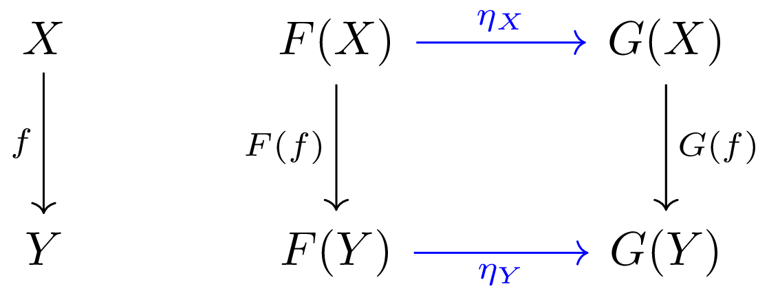
Each morphism \( \eta_X \) is called the component of \( \eta \) at \( X \) or the \( X \) component of \( \eta \).
5.2. Natural Isomorphism
- Natural Equivalence, Isomorphism of Functors
For every object \(X\) in \(\mathcal{C}\), the morphism \(\eta_X\) is an isomorphism in \(\mathcal{D}\).
5.3. Vertical Composition
Two natural transformations \( \eta\colon F\Rightarrow G \) and \( \epsilon\colon G\Rightarrow H \) between functors \( F, G, H\colon \mathcal{C} \to \mathcal{D} \) can be composed component-wise: \[ \epsilon \circ \eta\colon F \Rightarrow H, \quad (\epsilon\circ \eta)_X = \epsilon_X\circ \eta_X. \]
The name comes from the vertical arrangement of natural transformations in
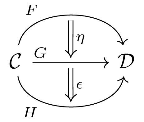
where the composed natural transformation is "longer".
5.4. Horizontal Composition
The two natural transformation \( \eta\colon F \Rightarrow G \) and \( \epsilon\colon J \Rightarrow K \) with \( F, G\colon \mathcal{C} \to \mathcal{D} \) and \( J, K\colon \mathcal{D} \to \mathcal{E} \), can be composed using the functor composition: \[ \epsilon * \eta\colon J\circ F \Rightarrow K \circ G, \quad (\epsilon*\eta)_X = \epsilon_{G(X)}\circ J(\eta_X) = K(\eta_X) \circ \epsilon_{F(X)}. \]
The composition makes the composed natural transformation "wider".
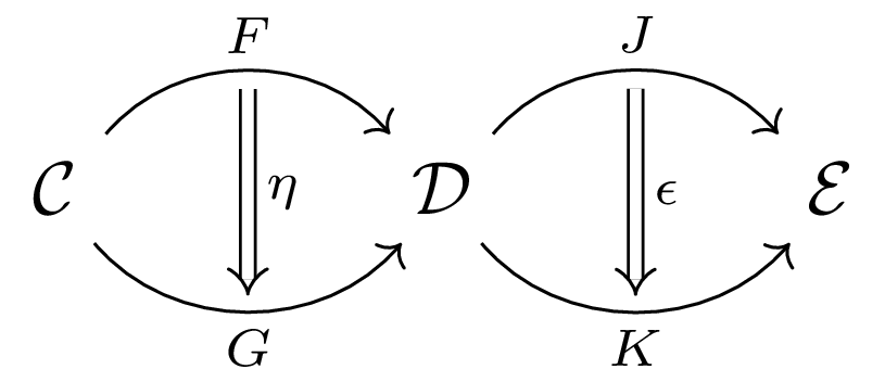
The horizontal composition is easily understood by a commutative diagram.
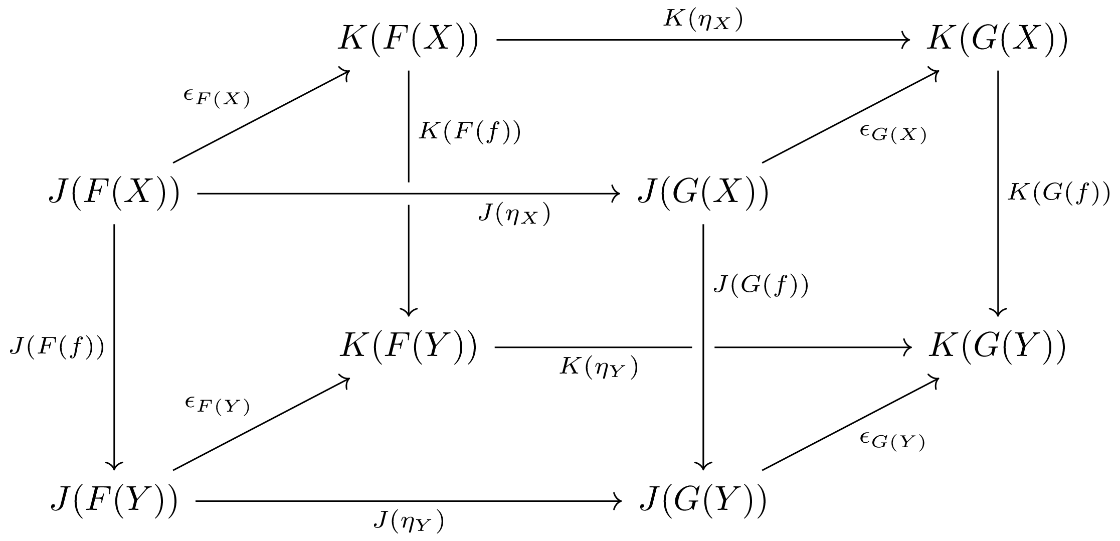
This is one step further from the commutative diagram in the definition of a natural transformation. Notice that the horizontal composition is nothing but the natural isomorphism from the \( J\circ F \) "column" to the \( K\circ G \) "column".
Whiskering can be used to simplify the notation. It is a binary operation between a functor and a natural transformation:
\begin{align*} J\eta\colon J\circ F \to J \circ G, \quad (J\eta)_X &:= J(\eta_X), \\ \eta J\colon J\circ F \to K \circ F, \quad (\eta J)_X &:= \eta_{J(X)}.\\ \end{align*}In light of whiskering, we can write \( \epsilon * \eta = \epsilon G \circ J\eta = K\eta\circ \epsilon F \), where \( \circ \) is the vertical composition.
5.5. Interchange Law
The vertical composition and horizontal composition interchange in the diagram:
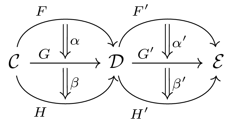
\( (\beta' \circ \alpha') * (\beta \circ \alpha ) = (\beta' * \beta) \circ (\alpha' * \alpha) \).
It can be seen relatively easily in the commutitive diagram with the shape of 3×3×2 cuboid.
6. Product
- \[ X_1 \times X_2 \]
A product of two objects \(X_{1}\) and \(X_{2}\) is an object \(X_{1}\times X_{2}\), such that for every object \(Y\) and every morphisms \(f_1\) and \(f_2\), there exists a morphism \(f\) that satisfies the following commutative diagram:

- "The smallest object that contains both object"
6.1. Coproduct
A coproduct of two objects \(X_{1}\) and \(X_{2}\) is an object \(X_{1}\oplus X_{2}\) (also written as \(X_1\sqcup X_2\), \(X_1\coprod X_2\) or \(X_1 + X_2\)), such that for every object \(Y\) and every morphisms \(f_1\) and \(f_2\), there exists a unique morphism \(f\) that makes the following diagram commutes:

7. Equaliser
The limit \((E, \mathrm{eq})\) of the morphisms \((Z, h)\) in the following diagram:
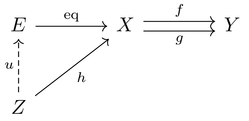
It equalises \( f \) and \( g \) in the sense that \(\mathrm{eq}[E] = \{x\in X \mid f(x) = g(x)\}\).
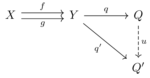
7.1. Coequaliser
Coequaliser is a colimit \((Q, q)\) of the diagram
8. Diagram
Diagram of type \(\mathcal{J}\) in a category \(\mathcal{C}\) is a covariant functor \( F\colon \mathcal{J}\to \mathcal{C} \) where \(\mathcal{J}\) is often a small or finite category.
\( \mathcal{J} \) called the index category or the scheme or the shape.
9. Limit
The limit of the diagram \(F\colon \mathcal{J}\to \mathcal{C}\) is a cone \((L, \{\phi_X\})\) to \(F\) such that factors every cone \((N, \{\psi_X\})\) by a unique morphism called the mediating morphism \(u\colon N\to L\)
.svg)
- This can be understood as the aptest cone that is universal.
9.1. Examples
- If \( \mathcal{J} \) is a discrete category, the limit is the product.
- If \( \mathcal{J} \) looks like \( \bullet \rightrightarrows \bullet \), the limit is the equaliser.
- If \( \mathcal{J} \) looks like \( \bullet \rightarrow \bullet \leftarrow \bullet \), the limit is the the pullback.
9.2. Colimit
Colimit is the limit in the opposite category.
10. Universal Property
- The relational property that uniquely determines an object up to isomorphism, since the category theory does not deal with the internal structure of an object.
- A property that is satisfied over all concrete contructions of the objects and morphisms.
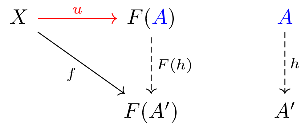
A universal morphism from \(X\) to \(F\colon \mathcal{C} \to \mathcal{D}\) is a unique pair \((A, u\colon X\to F(A))\) in \(\mathcal{D}\), which has the following property called universal property:
- For any morphism \( f \), there exists a unique morphism \( h \) such that the following diagram commutes
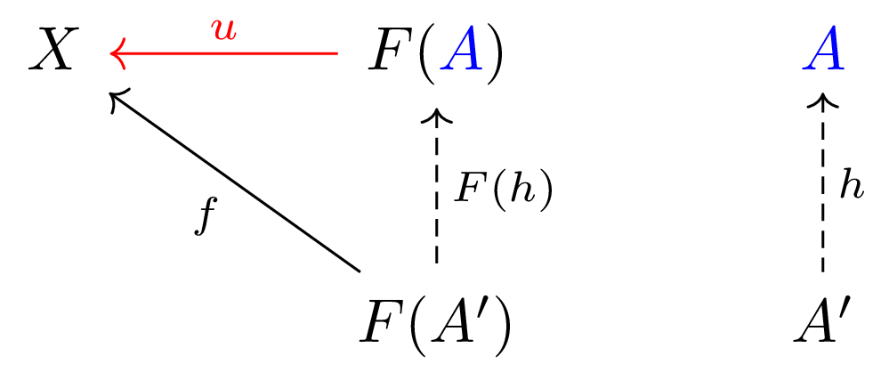
Similarly, a universal morphism from \( F \) to \( X \) is a unique pair \( ( A, u\colon F(A) \to X ) \) that satifies the following universal property:
- For any morphism \( f \), there exists a unique morphism \( h \) such that the following diagram commutes:
10.1. Examples
- The limit of a diagram \( F\colon \mathcal{J} \to \mathcal{C} \) is
the universal morphism from the diagonal functor \( \Delta\colon \mathcal{C} \to \mathcal{C}^{\mathcal{J}} \) to \( F \).
- The diagram is represented by the functor \( F \) and the limit cone (cone that is also the limit) is compressed into the natural transformation between the constant functor \( \Delta(\lim F) \) to \( F \).
- Similarly, the colimit of \( F\colon \mathcal{J} \to \mathcal{C} \) is a universal morphism from \( F \) to \( \Delta \).
- The tensor algebra \( T(V)\in K\text{-} \mathbf{Alg} \) of a vector space \( V \in K\text{-}\mathbf{Vect} \) over a field \( K \), with the inclusion map \( \iota\colon V \to U(T(V)) \) where \( U\colon K\text{-} \mathbf{Alg} \to K\text{-} \mathbf{Vect}\) is a forgetful functor, is the universal morphism from \( V \) to \( U \).
11. Yoneda Lemma
11.1. Statement
In a locally small category \( \mathcal{C} \), given a functor \( F: \mathcal{C} \to \mathbf{Set} \), and any object \( A \in \mathcal{C} \), there is one-to-one correspondence between natural transformations from the hom functor to \( F \), and the elements of \( F(A) \):
\begin{equation*} \mathrm{Hom}(\mathrm{Hom}(A,-), F) \cong F(A). \end{equation*}Informally, every property of the object \( A \) is recoverable by considering many morphisms from objects \( X \) to \( A \), \( \{X\to A\} \).
11.2. Proof
A natural transformation \( \Phi \) is completely determined by choosing \( u \in F(A) \) that \( \mathrm{id}_A \in \mathrm{Hom}(A,A)\) maps to.

11.3. Examples
- \( \{\mathbf{1}\to A\} \) is isomorphic to \( \mathrm{ob}(A) \).
- \( \{(0,1)\to A\} \) is every open set in \( A \) .
12. Sheaf
12.1. Presheaf
A presheaf \( F \) is a contravariant functor from a posetal category \( \mathcal{C} \) to \( \mathbf{Set} \).
12.2. Sheaf
A sheaf \( F \) is a presheaf that for every open cover \( \{U_i\} \) of any open set \( U \) \( F(U) \) is an in the following diagram: \[ F(U) \overset{f}{\to} \prod_i F(U_i) \overunderset{g}{h}{\rightrightarrows} \prod_{i,j} F(U_i\cap U_j) \] where \( f \) is the product of the restriction maps \[ f := \prod_ir^U_{U_i}\colon \sigma \mapsto (\sigma|_{U_1}, \sigma|_{U_2}, \dots) \] and \( g, h \) are the product of further restrictions
\begin{align*} g &:= \prod_{i,j} r^{U_i}_{U_i\cap U_j}, \\ h &:= \prod_{i,j} r^{U_j}_{U_i\cap U_j}. \end{align*}Intuitively, \( F(U) \) is all the continuous functions that is defined piecewise on each \( U_i \), provided that the pieces match at their intersections \( U_i\cap U_j \).
12.2.1. Properties
Due to the very definition of equalizer, a sheaf always has two properties: For any open set \( U\in X \), and for all open cover \( \{U_i\}_{i\in I} \) of \( U \) with \( \bigcup U_i = U \),
- Locality: \( \forall \sigma, \tau \in F(U)\colon \sigma = \tau \iff \forall i \in I, \sigma|_{U_i} = \tau|_{U_i}, \)
Gluing:
\begin{align*} \forall \{ \sigma_i \in &F(U_i)\}_{i\in I}\colon \\ &\forall i,j \in I, \sigma_i|_{U_i\cap U_j} = \sigma_j|_{U_i\cap U_j} \\ \implies &\exists \sigma \in F(U), \forall i \in I, \sigma|_{U_i} = \sigma_i. \end{align*}
12.3. Sheafification
The natural functor from the category of presheaf \( \mathbf{PSh}(\mathcal{C}) \) to the category of sheaf \( \mathbf{Sh}_J(\mathcal{C}) \). What is considered "natural" is dependent on the structure called coverage \( J \) of the posetal category \( \mathcal{C} \).
13. Monad
13.1. Definition
A monad is a triple \( (T, \eta, \mu) \) consisting of a endofunctor \( T\colon \mathcal{C} \to \mathcal{C} \) and two natural transformations \( \eta\colon 1_{\mathcal{C}} \to T, \mu\colon T^2 \to T \), where \( 1_{\mathcal{C}} \) is the identity functor, that satisfies the following commutative diagrams:
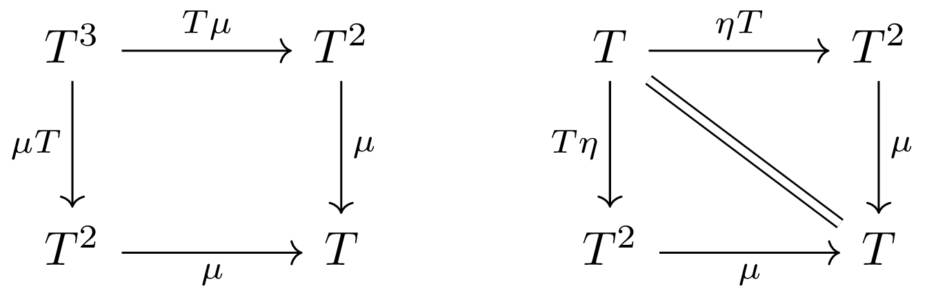
The first diagram is asserting the associativity of binary operation \( \mu \), and the second diagram is asserting the existence of an identity element \( \eta(1_{\mathcal{C}}) \) of the operation \( \mu \). Thus "monoid in the (monoidal) category of endofunctors (under composition)", with the understanding of monoid in the category theoretic sense.
13.2. Examples
- In functional programming, the
Maybemonad is an endofunctor on the category of types.
13.3. Kleisli Category
Given a monad \( (T, \eta, \mu) \) on a category \( \mathcal{C} \), the Kleisli category \( \mathcal{C}_T \) of \( \mathcal{C} \) can be constructed as follows:
\begin{align*} & \mathrm{ob}(\mathcal{C}_T) := \mathrm{ob}(\mathcal{C}), \\ & \mathrm{Hom}_{\mathcal{C}_T}(X,Y) := \mathrm{Hom}_{\mathcal{C}}(X, TY) \end{align*}and the composition of morphisms \( f\colon X\to TY \) and \( g\colon Y\to TZ \) is given by \[ g\circ_T f := \mu_Z \circ Tg \circ f\colon X \to TY \to T^2Z \to TZ \] with the identity morphism being \( \eta_X \).
Computer scientists often refer to Kleisli category
as the "monad".
They are also inclined to say that the function composition is the bind.
But technically, the function composition \( f \circ_T g \) is given as bind g . f, for example in Haskell.
See the embedding of Kleisli category for detail about bind.
13.4. Eilenberg-Moore Category
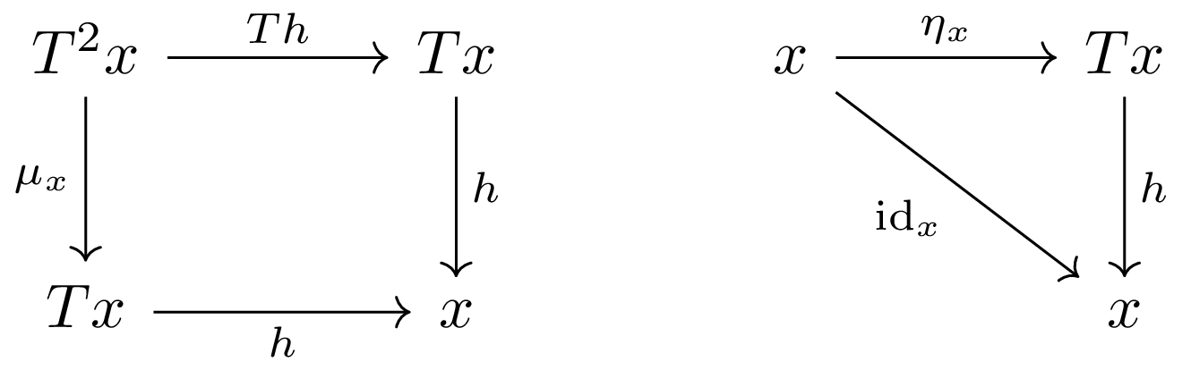
Given a monad \( (T, \eta, \mu) \) on a category \( \mathcal{C} \), the Eilenberg-Moore category \( \mathcal{C}^T \) can be constructed. The objects of \( \mathcal{C}^T \) are the \( T \)-algebras \( (x,h) \) where \( x \) is an object of \( \mathcal{C} \) and structure map of the algebra \( h\colon Tx \to x \) that makes the following diagrams commute:
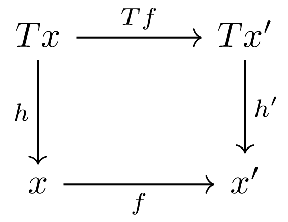
The morphism \( f\colon (x,h) \to (x', h') \) of \( T \)-algebras is the morphism \( f\colon x\to x' \) such that the following diagram commutes:
13.4.1. Embedding of Kleisli Category
The Kleisli category can be fully faithfully embedded into the Eilenberg-Moore category
with the embedding \( F: \mathcal{C}_T \to \mathcal{C}^T\colon X\mapsto (TX, \mu_X)\colon (f\colon X \to TY) \mapsto (\mu_Y\circ Tf\colon TX \to TY) \).
This mapping of the morphisms is also known as the bind map in functional programming.
14. Monoidal Category
- \( (\mathcal{C}, I, \otimes) \)
14.1. Monoid
A monoid \( (M, \eta, \mu) \) in a monoidal category \( (\mathcal{C}, I, \otimes) \) is an object \( M\in \mathcal{C} \) equipped with two morphisms \( \eta, \mu \) that satisfies the pentagon diagram and unitor diagram.
15. See Also
- Categorification of Fourier Theory - YouTube
- Category is the set of structures that share some properties.
16. References
- It is an abstraction of composition. The Mathematician's Weapon | An Intro to Category Theory, Abstraction and Alg…
- The definition. The Language of Categories | Category Theory and Why We Care 1.1 - YouTube
- Product. Universal Construction | Category Theory and Why We Care - YouTube
- Category theory - Wikipedia
- Natural transformation - Wikipedia
- Equaliser (mathematics) - Wikipedia
- Universal property - Wikipedia
- Diagram (category theory) - Wikipedia
- Limit (category theory) - Wikipedia
- Kan Academy: Introduction to Limits - YouTube
- Kan Academy: Intro to Colimits - YouTube
- Yoneda lemma - Wikipedia
- Sheaf (mathematics) - Wikipedia
- category of sheaves in nLab
- WTF is Sheafification?? - YouTube
- Monad (category theory) - Wikipedia
- What is a Monad? – Math vs Computer Science - YouTube